# A tibble: 5 × 4
       a       b     c       d
   <dbl>   <dbl> <dbl>   <dbl>
1  1.08  -1.46   0.243  0.239
2  1.02   0.0941 0.431 -0.0970
3 -1.83   0.310  1.38  -0.841
4 -0.164 -0.769  0.276 -1.01
5 -0.287 0.129 0.908 0.121 Functions
Day 16
Prof Emily Kurtz
Carleton College
Stat 220 - Spring 2026
Today
Writing Functions
Conditional Execution
Warm up
What does the mutate code below do?
Rescaling variables
Standardizing/rescaling/normalizing variables is often an essential first step in predictive modeling
Example:
Set of digitized breast cancer image features
Each row in the data set represents an image of a tumor sample, including the diagnosis (benign or malignant) and several other measurements (nucleus texture, perimeter, area, etc.)
Diagnosis for each image was conducted by physicians.
# A tibble: 569 × 12
        ID Class Radius Texture Perimeter  Area Smoothness Compactness Concavity
     <dbl> <chr>  <dbl>   <dbl>     <dbl> <dbl>      <dbl>       <dbl>     <dbl>
 1  8.42e5 M       18.0    10.4     123.  1001      0.118       0.278     0.300
 2  8.43e5 M       20.6    17.8     133.  1326      0.0847      0.0786    0.0869
 3  8.43e7 M       19.7    21.2     130   1203      0.110       0.160     0.197
 4  8.43e7 M       11.4    20.4      77.6  386.     0.142       0.284     0.241
 5  8.44e7 M       20.3    14.3     135.  1297      0.100       0.133     0.198
 6  8.44e5 M       12.4    15.7      82.6  477.     0.128       0.17      0.158
 7  8.44e5 M       18.2    20.0     120.  1040      0.0946      0.109     0.113
 8  8.45e7 M       13.7    20.8      90.2  578.     0.119       0.164     0.0937
 9  8.45e5 M       13      21.8      87.5  520.     0.127       0.193     0.186
10  8.45e7 M       12.5    24.0      84.0  476.     0.119       0.240     0.227
11  8.46e5 M       16.0    23.2     103.   798.     0.0821      0.0667    0.0330
12  8.46e7 M       15.8    17.9     104.   781      0.0971      0.129     0.0995
13  8.46e5 M       19.2    24.8     132.  1123      0.0974      0.246     0.206
14  8.46e5 M       15.8    24.0     104.   783.     0.0840      0.100     0.0994
15  8.47e7 M       13.7    22.6      93.6  578.     0.113       0.229     0.213
16  8.48e7 M       14.5    27.5      96.7  659.     0.114       0.160     0.164
# ℹ 553 more rows
# ℹ 3 more variables: Concave_Points <dbl>, Symmetry <dbl>,
#   Fractal_Dimension <dbl>
Standardizing variables
Goal: standardize the 10 quantitative variables in the data set
Approach: subtract sample mean, divide by sample standard deviation
scaled_cancer <- unscaled_cancer %>%
  mutate(
    Radius = (Radius - mean(Radius)) / sd(Radius),
    Texture = (Texture - mean(Texture)) / sd(Texture),
    Perimeter = (Perimeter - mean(Perimeter)) / sd(Perimeter),
    Area = (Area - mean(Area)) / sd(Area),
    Smoothness = (Smoothness - mean(Smoothness)) / sd(Smoothness),
    Compactness = (Compactness - mean(Compactness)) / sd(Compactness),
    Concavity = (Concavity - mean(Concavity)) / sd(Concavity),
    Concave_Points = (Concave_Points - mean(Concave_Points)) / sd(Concave_Points),
    Symmetry = (Symmetry - mean(Symmetry)) / sd(Symmetry),
    Fractal_Dimension = (Fractal_Dimension - mean(Fractal_Dimension)) / sd(Fractal_Dimension)
  )
Don’t repeat yourself (DRY)
We’ve copied, pasted, and edited the same code chunk many times
That’s a lot of work when the only change in the code is the variable name!
scaled_cancer <- unscaled_cancer %>%
  mutate(
    Radius = (Radius - mean(Radius)) / sd(Radius),
    Texture = (Texture - mean(Texture)) / sd(Texture),
    Perimeter = (Perimeter - mean(Perimeter)) / sd(Perimeter),
    Area = (Area - mean(Area)) / sd(Area),
    Smoothness = (Smoothness - mean(Smoothness)) / sd(Smoothness),
    Compactness = (Compactness - mean(Compactness)) / sd(Compactness),
    Concavity = (Concavity - mean(Concavity)) / sd(Concavity),
    Concave_Points = (Concave_Points - mean(Concave_Points)) / sd(Concave_Points),
    Symmetry = (Symmetry - mean(Symmetry)) / sd(Symmetry),
    Fractal_Dimension = (Fractal_Dimension - mean(Fractal_Dimension)) / sd(Fractal_Dimension)
  )
You should consider writing a function
whenever you’ve copied and pasted a
block of code more than twice
—Hadley Wickham
Why functions?
Automate common tasks in a more powerful and more general way than copy-and-pasting
You can give a function an evocative name that makes your code easier to understand.
As requirements change, you only need to update code in one place, instead of many.
You eliminate the chance of making incidental mistakes when you copy and paste (i.e. updating a variable name in one place, but not in another).
Down the line — Improve your reach as a data scientist by writing functions (and packages!) that others use
Anatomy of a function
Anatomy of a function
Anatomy of a function
Building standardize
Building standardize
Building standardize
Does it work?
Unstandardized Compactness
Standardized Compactness from copy and paste mutate() code
Your turn
Turn the following code snippets into functions. Think about what each function does before you begin (think SI vs. imperial units), and be sure to give each function an informative name.
x * 0.0022x / sum(x, na.rm = TRUE)
You can test your functions on variables from the palmerpenguins::penguins dataset (e.g. my_func(penguins$body_mass_g)).
Return values
The value returned by the function is usually the last statement it evaluates
Adding arguments
We can include na.rm as an argument to give the user control over it
Setting defaults
Unless a default value is set for an argument, R will require a value to be specified in the function call
 Error in mean(x, na.rm = na.rm) :
  argument "na.rm" is missing, with no default
Setting defaults
To set a default, set the value in the function definition
  [1] -0.563316704 -0.500969030 -1.186793445           NA -0.937402749
  [6] -0.688012052 -0.719185889  0.590115266 -0.906228912  0.060160036
 [11] -1.124445771 -0.625664378 -1.249141119 -0.500969030  0.247203059
 [16] -0.625664378 -0.937402749  0.371898407 -1.093271934 -0.002187638
 [21] -0.999750423 -0.750359726 -0.500969030 -0.313926008 -0.500969030
 [26] -0.500969030 -0.812707400 -1.249141119 -1.311488793 -0.313926008
 [31] -1.186793445 -0.376273682 -1.124445771 -0.376273682 -1.093271934
 [36] -0.064535312 -0.313926008 -0.812707400 -1.124445771  0.558941429
 [41] -1.311488793 -0.376273682 -1.373836467  0.247203059 -1.498531815
 [46]  0.496593755 -0.968576586 -1.529705652 -0.937402749 -0.064535312
 [51] -0.875055074  0.122507710 -0.937402749 -0.189230660 -1.623227163
 [56] -0.625664378 -0.812707400 -0.500969030 -1.685574837 -0.563316704
 [61] -1.311488793  0.247203059 -0.750359726 -0.189230660 -1.685574837
 [66] -0.313926008 -1.062098097 -0.126882986 -1.436184141  0.309550733
 [71] -0.750359726 -0.376273682 -0.812707400 -0.064535312 -0.625664378
 [76]  0.060160036 -0.625664378 -0.376273682 -0.812707400 -0.251578334
 [81] -1.249141119  0.621289103 -0.500969030 -0.002187638 -1.062098097
 [86] -0.812707400 -0.500969030 -0.875055074 -0.313926008 -0.750359726
 [91] -0.812707400  0.122507710 -0.999750423  0.309550733 -1.124445771
 [96]  0.122507710 -0.625664378  0.184855384 -1.623227163 -0.126882986
[101] -0.594490541  0.652462940 -1.405010304  0.060160036 -1.592053326
[106] -0.812707400 -0.563316704 -0.376273682 -1.280314956  0.714810614
[111] -0.469795193  0.496593755 -1.249141119  0.091333873 -0.376273682
[116] -0.158056823 -1.623227163 -0.532142867 -1.062098097 -1.093271934
[121] -1.311488793 -0.875055074 -0.937402749 -0.407447519 -1.436184141
[126] -0.251578334 -1.155619608  0.122507710 -1.436184141 -0.251578334
[131] -1.093271934 -0.875055074 -0.875055074  0.340724570 -0.968576586
[136] -0.376273682 -1.280314956 -0.282752171 -0.999750423  0.060160036
[141] -0.999750423 -0.906228912 -1.436184141 -0.594490541 -1.498531815
[146] -0.688012052  0.060160036 -0.906228912 -0.937402749 -0.563316704
[151] -0.625664378 -0.251578334  0.371898407  1.868242584  0.309550733
[156]  1.868242584  1.494156540  0.434246081  0.745984451  1.244765843
[161]  0.247203059  1.182418169  0.558941429  1.681199562  0.558941429
[166]  2.055285606 -0.002187638  2.055285606 -0.064535312  2.616414673
[171]  0.745984451  1.431808866  1.868242584  0.995375147  0.247203059
[176]  1.057722821  0.995375147  1.120070495 -0.126882986  1.805894910
[181]  0.496593755  1.681199562  1.307113518  0.621289103  1.057722821
[186]  2.304676302  1.182418169  1.494156540  0.933027473  1.307113518
[191]  0.184855384  1.431808866 -0.313926008  1.868242584  0.122507710
[196]  0.683636777  1.681199562  0.870679799 -0.002187638  1.494156540
[201]  1.120070495  1.369461192  0.808332125  1.369461192  0.247203059
[206]  0.995375147  0.870679799  1.057722821  0.122507710  0.995375147
[211]  0.309550733  1.681199562 -0.002187638  1.369461192  0.247203059
[216]  1.805894910  0.621289103  1.868242584  0.558941429  1.992937932
[221]  0.621289103  1.681199562  0.683636777  0.995375147  1.120070495
[226]  1.244765843  0.621289103  1.992937932  0.496593755  2.242328628
[231]  0.683636777  2.179980954  0.527767592  1.556504214  0.652462940
[236]  1.431808866  0.683636777  1.743547236  0.496593755  1.369461192
[241]  0.839505962  1.681199562  0.933027473  1.494156540  0.683636777
[246]  1.805894910  0.808332125  1.244765843  0.901853636  0.839505962
[251]  0.527767592  1.307113518  0.808332125  1.743547236  0.964201310
[256]  1.618851888  0.652462940  1.618851888  0.621289103  1.618851888
[261]  0.465419918  1.618851888  0.995375147  2.179980954  0.558941429
[266]  1.618851888  0.216029222  2.055285606  0.839505962  2.242328628
[271]  0.901853636           NA  0.808332125  1.930590258  1.244765843
[276]  1.494156540 -0.875055074 -0.376273682 -0.688012052 -0.843881237
[281] -0.594490541 -0.313926008 -1.186793445 -0.563316704 -0.064535312
[286] -0.625664378 -0.500969030 -0.532142867 -0.625664378 -0.189230660
[291] -0.781533563 -0.189230660 -1.124445771 -0.625664378 -0.937402749
[296]  0.247203059 -0.750359726 -0.999750423 -1.623227163 -0.500969030
[301] -1.124445771 -0.064535312 -0.999750423 -0.500969030 -0.625664378
[306]  0.434246081 -1.249141119  0.122507710 -1.062098097 -0.126882986
[311] -0.750359726 -0.376273682 -0.438621356  0.745984451 -1.872617859
[316]  0.371898407 -0.313926008 -0.688012052 -0.812707400 -0.875055074
[321] -0.656838215  0.309550733 -0.999750423  0.122507710 -1.186793445
[326] -0.656838215 -1.093271934 -0.313926008 -0.750359726 -0.189230660
[331] -1.062098097 -0.937402749 -1.186793445 -0.189230660 -0.500969030
[336] -0.843881237 -0.313926008 -0.688012052 -0.688012052 -0.251578334
[341] -0.999750423 -0.532142867 -0.126882986 -0.532142867
Your turn
Write a function called
column_meanthat takes a data set and column name (as a string) as inputs and returns the column mean as output. (Hint: access the column using[[)You should also include a
na.rmargument and set the default toTRUEso thatNAs are removed from the calculation by default.Test your function on the
mtcarsdata set.
Plotting functions
p1 = unscaled_cancer %>%
  ggplot(aes(x = Radius, fill = Class)) +
  geom_histogram(col = "white", bins = 20, alpha = .7)

p2 = unscaled_cancer %>%
  ggplot(aes(x = Texture, fill = Class)) +
  geom_histogram(col = "white", bins = 20, alpha = .7)

p3 = unscaled_cancer %>%
  ggplot(aes(x = Perimeter, fill = Class)) +
  geom_histogram(col = "white", bins = 20, alpha = .7)

p4 = unscaled_cancer %>%
  ggplot(aes(x = Area, fill = Class)) +
  geom_histogram(col = "white", bins = 20, alpha = .7)

(p1 + p2)/(p3 + p4)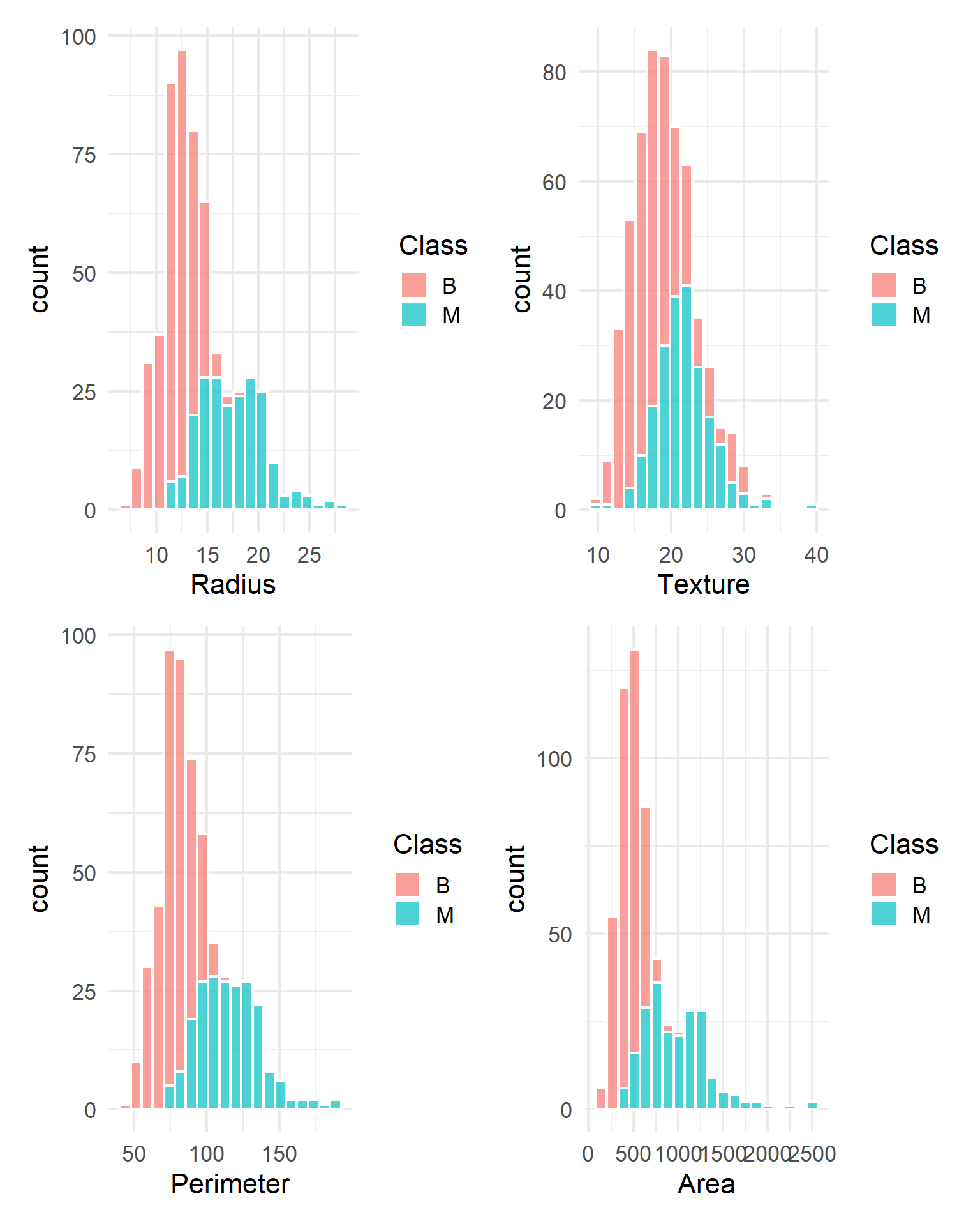
Custom histogram() function
Error in `geom_histogram()`:
! Problem while computing aesthetics.
ℹ Error occurred in the 1st layer.
Caused by error:
! object 'Radius' not found
🤗 embracing 🤗
This issue arises in {dplyr} and {ggplot} functions because they use a special kind of evaluation, which allows us to refer to our variable names directly when writing code with their functions.
To write our own functions that use these packages, we use 🤗 embracing 🤗 (wrap the variable in braces). This tells R to use the value stored inside the argument, not the argument as the literal variable name.
Ex:
count(my_variable) looks for a column literally named my_variable
count({{my_variable}}) looks for the column name stored inside my_variable
histogram() function

Your turn
Write a plotting function called scatterplot() that makes a scatterplot of any two quantitative variables, coloring the points by a 3rd categorical variable.
Test your function with the following examples:


Functions with conditional execution
- Sometimes, we want our function to do different things depending on the arguments we feed it.
- Example: a
histobarfunction that makes ahistogram if the variable is quantitative and abarchart if the variable is categorical.


Conditional execution
The if() statement allows us to control which statements are executed.
Conditional execution
A basic example
[1] 5Conditional execution
Another basic example
[1] 4histobar
Error: object 'Radius' not foundhistobar
{var} is a column in a data frame/tibble, but is.numeric only works on vectors
histobar
pull() works like a $
Testing histobar
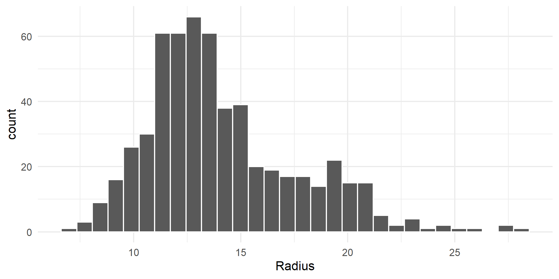
Testing histobar
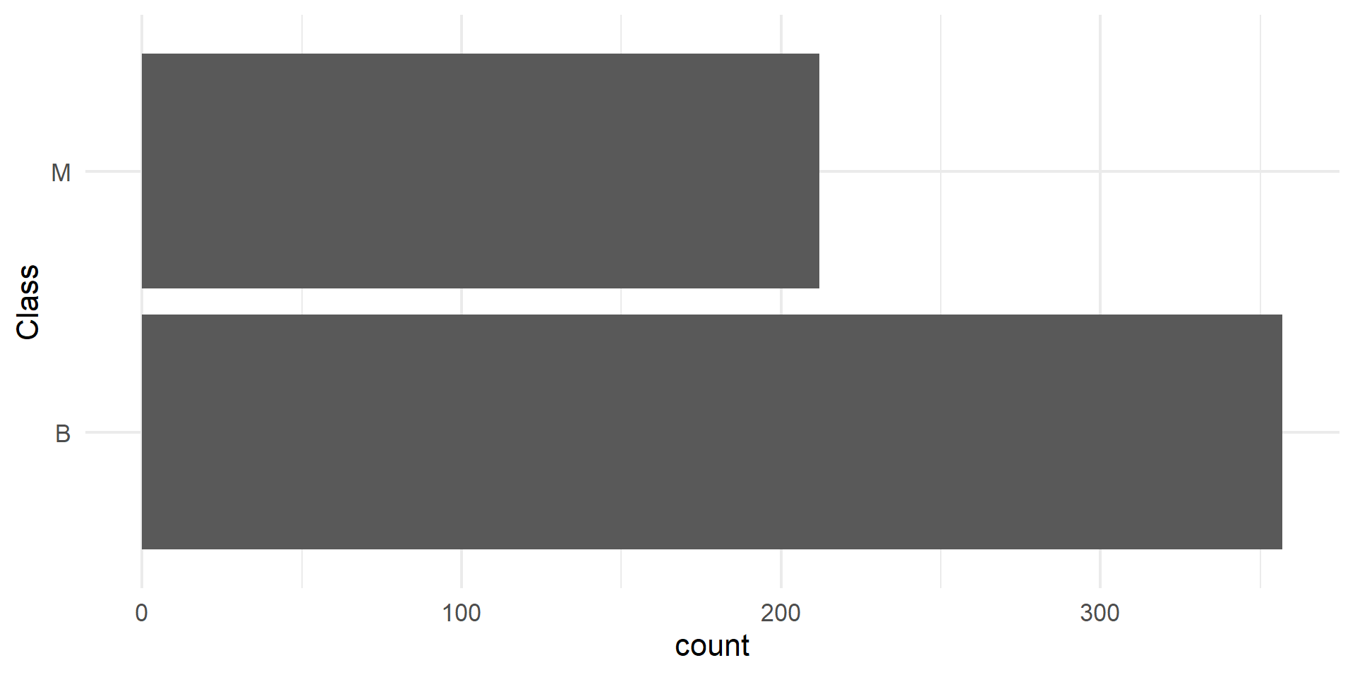
Testing histobar
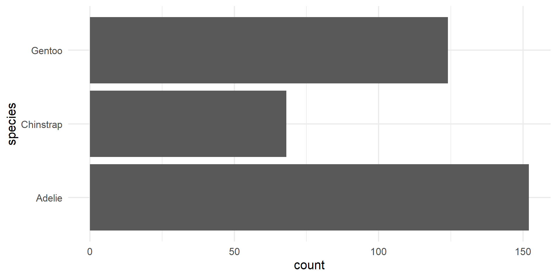
Testing histobar
Your turn
Edit your scatterplot function to include an argument called draw_line. If draw_line is TRUE, your function should add a line of best fit to your scatterplot. Test your function with the following examples

